Understanding Attention by Tracing Its Origins

1Introduction

A few weeks back, I was trying to learn the transformer attention mechanism. I found that most articles teach attention by just stating its formula and how it’s used in inference, but the formula only makes sense once you understand the failure it was designed to fix.

One path forward was to understand attention as an abstraction and start learning subsequent things. But that felt shallow. I traced the origins back to pioneering research papers to understand how it came into existence and how it evolved into the attention most transformers use today.

This blog serves as a note of my understanding.

2The problem before the attention

2.1RBMT / SMT

In NLP, the problem that led to the development of attention-based transformers was translation. Before neural machine translation (NMT) with attention (popularized around 2014–2017), translation systems were dominated by statistical and rule-based approaches.

One such approach is Rule-Based Machine Translation (RBMT), which predates 2010. It used rule-based grammar (as the name suggests). Linguists manually created grammar rules, dictionaries, and transfer rules between languages. It had good interpretability, but it was extremely labor-intensive, hard to scale to many languages, and brittle with ambiguous or informal text.

Another approach was Statistical Machine Translation (SMT). It was the most prevalent solution before neural models. The core idea was to treat translation as a probability problem to find the target sentence $e$ that maximises:

where $f$ is the source sentence, $e$ is the target sentence, $P(f|e)$ is the translation model, and $P(e)$ is the language model. There were a few different variants of SMT. Word-Based SMTs learned word alignments and modeled translation word-by-word, but they couldn’t capture idioms well. A more powerful version was Phrase-based SMT that would translate chunks of text and stitch them together into the most fluent sentence possible.

These systems relied on explicit alignment heuristics rather than learning alignment end-to-end from data. These systems had a clear limitation; they treated alignment and translation as separate problems. Neural models promised to learn both jointly.

2.2Seq2Seq (encoder-decoder)

Deep Neural Networks (DNN) have been powerful for tasks such as speech recognition and image classification. They are typically trained using supervised backpropagation with a large amount of labeled data. Backpropagation can learn parameters that perform well for a given problem.

One important limitation of DNNs (applicable to all standard feedforward neural networks) was that they required the inputs and outputs to be encoded into fixed-sized vectors. This limitation held DNNs back from solving an interesting set of problems that involved samples with variable input and output vectors. Such problems include machine translation, summarisation, and speech recognition, where we don’t know the lengths of sequences a priori. Thus, a domain-independent method was required that could learn an arbitrary sequence-to-sequence mapping.

Around that time, Sutskever et al. [1] proposed an LSTM-based encoder-decoder model. It was the first widely successful LSTM-based sequence-to-sequence Neural Machine Translation (NMT) system. The model takes variable-length input, maps it to a fixed-dimensional vector using the encoder LSTM, and then sequentially decodes the target sequence using that fixed-dimensional vector and the decoder LSTM. It was trained on the WMT’14 English-to-French translation dataset, which contains 12 million sentence pairs comprising 348 million French words and 304 million English words.

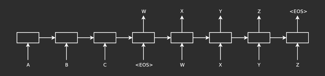
Figure 1: The model reads the input sequence “ABC” and produces “WXYZ” as output. Credit: Sutskever et al. [1].

Figure 1: The model reads the input sequence “ABC” and produces “WXYZ” as output. Credit: Sutskever et al. [1].

The LSTM estimates the conditional probability of an output sequence $(y_1, \ldots, y_{T'})$, given a set of input sequence $(x_1, \ldots, x_T)$, where both the input and output sequences can be of arbitrary length.$^1$

This discovery was groundbreaking at that time, but it had its own limitations.

1. The major one was that using a fixed-dimensional context vector was a bottleneck because it meant all the information from the input sequence must be compressed into a single fixed-dimensional vector. This means the model has no way to selectively focus on different parts of the input while generating each output token. When sentences became long, important words got lost, and translation quality dropped. This is a many-to-one non-linear compression, so the compression is deterministic, non-linear (due to LSTM/activation functions) and fixed.

   $$\R^{T \times d_x} \rarr \R^{d_h}$$

2. Another issue was that it had difficulty handling long-range word dependencies. Even though LSTMs were designed to mitigate vanishing gradients, early seq2seq models still struggled with very long sequences. The decoder relied heavily on the last encoder hidden state; the information from early parts of the input could fade and capturing long-distance relationships between words was unreliable. This means early tokens must survive through $T$ steps to form meaningful connection. This caused the LSTMs to miss context, use incorrect word order, and drop important words during translation. Empirically, performance degrades with sentence length.

3Attention: The First Attempt

3.1Mathematics behind RNN-based encoder-decoder

As mentioned previously, an RNN-based encoder-decoder needs to compress the source sentence information into a fixed-dimensional vector, which makes it difficult for the model to handle sentences longer than those seen during training. Cho et al. [3] showed that the performance of such an encoder-decoder model deteriorates as the length of the input increases.

From a probabilistic perspective, the task of translation can be modelled as maximising the conditional probability of predicting a target sequence $\bold{y}$ given an input sequence $\bold{x}$, expressed as $argmax_{\bold{y}} P(\bold{y}|\bold{x})$.

The RNN-based encoder-decoder model takes in a sequence of vectors $\bold{x} = (x_1, ..., x_{T_x})$ and compress it into a context vector $c$.

where $h_t$ is a hidden state at time $t$, and $c$ is a vector generated from a sequence of hidden states. The decoder is trained to predict the next word $y_{t’}$ given the context vector $c$ and previously predicted tokens $\{{y_1, …, y_{t’-1}}\}$ as input.

where $\bold{y} = (y_1,…, y_{T_y})$. Each conditional probability can be modeled as a nonlinear, multi-layered function $g$ that helps predict the probability of $y_t$. $s_t$ is the hidden state of RNN at time $t$.

3.2First Attempt at Attention

To address this issue of context compression, Bahdanau et al. [2] proposed a method that soft-searches for a set of positions in the source where the most relevant information is stored. The model uses this stored information and all the previously generated target words to generate the next word.

Unlike the RNN-based encoder-decoder model, [2] introduce a bidirectional RNN as an encoder and a decoder that emulates soft-search over the whole input during translation. They propose a novel decoder architecture that learns to align and translate simultaneously during training.

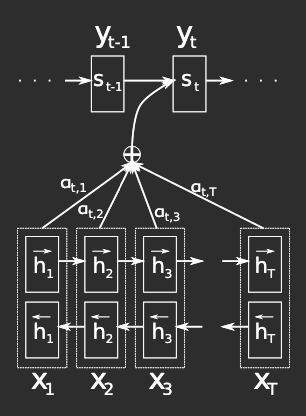
Figure 2: Model proposed by [2] trying to generate $t$-th target word $y_t$. Credit: Bahdanau et al. [2].

The proposed model defines the conditional probability as follows:

where $s_i$ is an RNN decoder hidden state for time $i$. Note that, unlike the previous encoder-decoder approach, the probability is conditioned on a distinct context vector $c_i$ for each target token $y_i$. The context vector $c_i$ is computed as a weighted sum of these annotations $h_i$. Each annotation $h_i$ encodes information about the full input sequence, with particular attention to the context near the 𝑖-th word.

The weight $\alpha_{ij}$ of each annotation $h_j$ is computed using softmax:

where

$e_{ij}$ is an alignment model that scores the inputs around position $j$ and outputs around position $i$ match. This scoring function is the core of attention - it quantifies how relevant each input position is for generating the current output. The score is computed using the RNN hidden state $s_{i-1}$ and the $j$-th annotation $h_j$ of the input sequence. The alignment model $a$ can be implemented as an FFNN and is trained jointly with the rest of the system.

The model treats alignment as a probability distribution and computes the context vector $c_i$ as the average (expectation) of all encoder states $(h_1,…,h_{T_x})$, weighted by how likely each one is relevant.

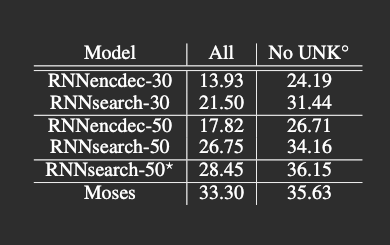
Table 1: The proposed model (RNNsearch*) performed much better than the conventional model (RNNencdec*) on both All (all sentences) and No UNK (on sentences without any unknown word in input and output). Credit: Bahdanau et al. [2].

This approach moved the frontier forward. Table 1 shows BLEU scores on the WMT’14 test set (news-test-2014) of 3,003 sentences unseen during training. RNNsearch surpasses RNNencdec and achieves comparable performance to Moses for sentences without unknown words (No UNK).

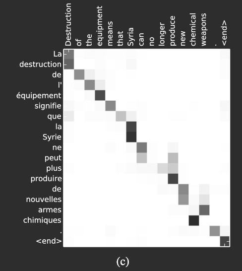
Figure 3: Shows the non-trivial, non-monotonic learned alignment between English and French words. Credit: Bahdanau et al. [2].

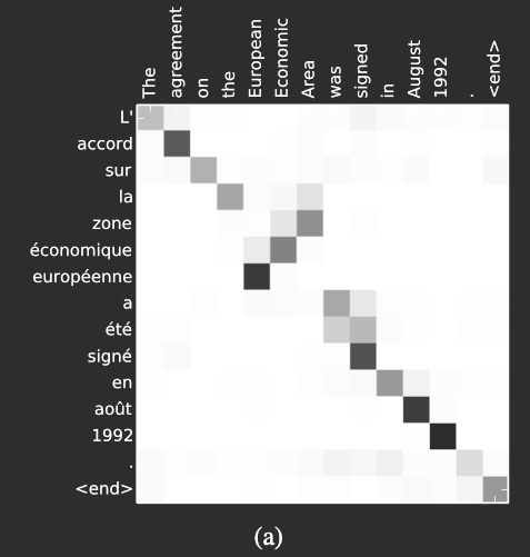
Figure 4: Shows the non-trivial, non-monotonic learned alignment between English and French words. Credit: Bahdanau et al. [2].

The word alignments between English and French are largely monotonic, which is reflected in the strong diagonal patterns in the alignment matrices in Figure 3. In many cases, this means the model maps words in roughly the same order across both languages.

However, Figure 3 also highlights some non-trivial, non-monotonic alignments. These arise from structural differences between the two languages, particularly in how adjectives and nouns are ordered.

For example, the phrase [European Economic Area] is translated into [zone économique européenne], where the word order differs from English. The model correctly aligns [zone] with [Area], even though it has to skip over [European] and [Economic] to do so. It then proceeds step by step to generate the full phrase [zone économique européenne].

This shows that the model is not limited to simple left-to-right alignment, but can also learn to handle reordering when required.

3.3Intuitions

The standard encoder–decoder model compresses the entire input sequence into a single fixed-dimensional vector $c$, creating an information bottleneck that becomes more severe as input length increases.

The attention-based model removes this constraint by introducing a time-dependent context vector $c_i$ (Eq. 3). Instead of relying on a single summary, the decoder computes $c_i$ at each step as a weighted sum of encoder annotations (Eq. 4), where the weights $\alpha_{ij}$ (Eq. 5) are determined by an alignment model $a(s_{i-1}, h_j)$ (Eq. 6).

This mechanism allows the model to dynamically select relevant parts of the input sequence for each output token. The alignment weights form a probability distribution over input positions, enabling the context vector to represent an expectation over encoder states rather than a fixed summary.

As a result, the model can handle long-range dependencies and non-monotonic alignments more effectively, since it is no longer constrained to encode all information into a single vector.

4Types of Attention

4.1Abstract Formulation

Bahdanau attention introduced a clear shift in how the problem is approached: instead of relying on a fixed representation, the model computes a context vector at each decoding step. This simple but powerful idea changed how sequence-to-sequence models handle information flow. In the following years, several variations of this mechanism were proposed. Although they differ in formulation, they can be understood through a common unifying abstraction.

In simple terms, the attention mechanism does the following at each decoding step:

All attention mechanisms can be written as :

Where

• $score$ is the alignment function
• $Q$ (query) is what we are looking for
• $K$ (keys) is what we match our query against (labels/descriptions of stored items)
• $V$ (values) is the actual content we want to retrieve

Different attention-based mechanisms use different $score$ functions with different $bias/mask$. But the overall structure remains the same.

Although early attention mechanisms were not described this way, we can reinterpret them using the modern Query-Key-Value (Q/K/V) framework.

4.2Additive Attention (Bahdanau et al.)

Additive Attention score function tells us how relevant the encoder hidden state $h_j$ is to the decoder at step $i$.

Here:

• Query ($Q$): previous decoder hidden state $s_{i-1}$
• Key ($K$): current encoder hidden state $h_j$
• Value ($V$): current encoder hidden state $h_j$

The alignment model $a(⋅)$ is a learned function that measures compatibility between the query and key. Bahdanau et al. [2] parameterize $a$ as a simple single-hidden-layer MLP:

where $W_s \in \mathbb{R}^{d_a \times d_s}$, $W_h \in \mathbb{R}^{d_a \times d_h}$, $v_a \in \mathbb{R}^{d_a}$, and $\phi = \tanh$

This gives the final attention scores and context vector:

• $W_ss_{i-1}$ projects the Query (decoder state) into the alignment space; changing $W_s$ to $W_q$
• $W_hh_j$ projects the Key (encoder state) into the same space; changing $W_h$ to $W_k$
• Their sum is passed through $\tanh$ to allow non-linearity
• Finally, $v^\top$ reduces the vector to a scalar score $e_{ij}$

In the common Q/K/V notation

4.3Multiplicative Attention (Luong et al.)

Luong et al. [5] introduce two attention approaches: global attention, which considers all source positions (similar to [2]), and local attention, which focuses on a subset of source positions. The local approach can be seen as a hybrid between hard and soft attention Xu et al. [7].

Unlike Bahdanau’s additive attention, which learns a compatibility function, Luong attention assumes that similarity in the representation space directly implies relevance. Both approaches take the decoder hidden state $h_t$ from the top LSTM layer and derive a context vector $c_t$ that summarizes relevant encoder information for predicting the current target token $y_t$.

Both approaches differ in how they calculate $c_t$, but the subsequent steps are similar. A simple concatenation layer is applied on decoder hidden state $h_t$ and $c_t$ to combine information from both the vectors to produce an attentional hidden state:

It is passed through a $softmax$ layer to produce a predictive distribution:

4.3.1Global Attention

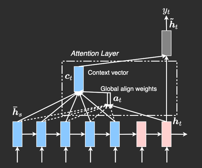
Figure 5: Global attentional model: At each time step $t$, variable-length alignment weights $a_t$ are computed from the current target state $h_t$ and all source states $\bar{h_s}$, producing a context vector $c_t$ as their weighted average. Credit: Luong et al. [5]

In global attention, all encoder hidden states are considered when computing the context vector $c_t$. The alignment weights are computed as:

where $score$ can be calculated as

[5]’s global attention is similar to [2] in spirit, but there are some key differences that make [5]’s global attention simpler. For instance, [5] relies only on the top LSTM layers in both the encoder and decoder. Its computation flow is also more straightforward, progressing from $h_t \rightarrow a_t \rightarrow c_t \rightarrow \tilde{h_t}$, then producing predictions. In contrast, [2] compute attention differently: at each time step $t$, they start from the previous hidden state, following the path $h_{t-1} \rightarrow a_t \rightarrow c_t \rightarrow h_t$. This output is then passed through additional components, including a deep-output layer and a maxout layer, before generating the final prediction.

Replacing the standard notation with Q/K/V for clarity:

The score function becomes:

Overall, the conventional attention formula will be

4.3.1.1 Intuition

Global attention identifies encoder states most similar to the current decoder state and averages them according to their similarity scores.

Luong’s multiplicative attention works well when the representation space already captures meaningful relationships, where similarity between vectors implies relevance. In contrast, Bahdanau’s additive attention learns how to compare vectors through a small neural network, capturing asymmetry and nonlinear feature interactions. In other words:

• Luong: compares vectors directly (geometry-based, like dot product).
• Bahdanau: learns what ‘relevance’ means (neural ranking).

4.3.2Local Attention

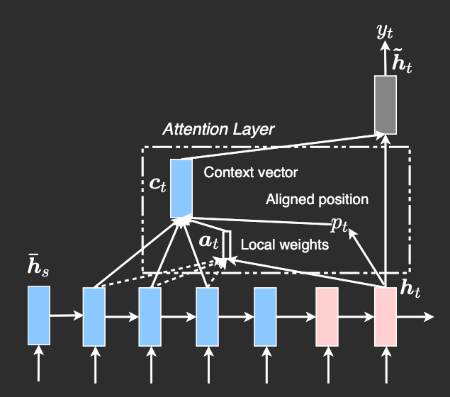
Figure 6: Local attention model: At each time step $t$, the model predicts an aligned position $p_t$ and computes the context vector $c_t$ as a weighted average over source states within a window around it, with weights $a_t$ derived from the current target state $h_t$. Credit: Luong et al. [5]

Attending to all encoder states at every decoding step can be computationally expensive, especially for long sequences. Local attention addresses this by restricting attention to a small subset of source positions for each target token.

At each decoding step $t$, the model predicts an aligned position $p_t$, and computes the context vector $c_t$ using only encoder states within a window $[p_t-D, p_t+D]$, where $D$ is a predefined window size. This makes the attention distribution $a_t$ fixed in size, with $a_t \in \R^{2D+1}$.

4.3.2.1 Alignment strategies

[5] propose two variants for determining $p_t$:

1. Monotonic alignment (local-m)

   Assumes source and target sequences are roughly aligned in order and set $p_t = t$. The attention weights ($a_t$) are then computed using the same scoring function as in global attention, restricted to the local window

2. Predictive alignment (local-p)

   Learns to predict the aligned position:

   $$p_t = S \cdot sigmoid(v_p^\top \tanh(W_p h_t))$$

   where $Wp$ and $v_p$ are learned parameters, and $S$ is the source sentence length.

We place a Gaussian distribution centered around $p_t$ to favor alignment points near $p_t$.

We use the same alignment function as global attention, and standard deviation is empirically set to $D/2$.

4.3.2.2 Attention computation

Using Q/K/V notation:

The attention weights are computed by combining three components:

1. Content-based score (same as global attention):

   $$score(Q, K)$$

2. Gaussian bias (soft preference towards $p_t$):

   $$B_{gaussian}(s) = -\frac{(s - p_t)^2}{2\sigma^2}$$

3. Window mask (hard constraint):

   $$M_{window}(s) = \begin{cases} 0 & s \in [p_t-D, p_t+D] \\ -\infty & \text{otherwise} \\ \end{cases}$$

The overall attention is:

For local-m, $p_t = t$ and the Gaussian bias is typically omitted, relying only on the window constraint.

4.3.2.3 Intuition

Local attention imposes two locality constraints:

• A hard constraint via the window, limiting which encoder states are considered
• A soft constraint via the Gaussian bias encouraging focus near $p_t$

This reduces computation while still allowing the model to focus on the most relevant region of the input. Compared to global attention, it trades full context for efficiency, while retaining flexibility through the learned alignment in the predictive variant.

5From Attention to Self-Attention

5.1Limitation of RNN + Attention

In sequence models, path length represents the number of steps information must travel to influence the output. As mentioned earlier in section 2.2, in plain RNN seq2seq, the information from early tokens must pass through $T$ sequential steps. This leads to vanishing gradients and difficulty remembering long-range dependencies.

Attention introduces a shortcut. At each decoding step, the model can directly access all encoder hidden states. This provides a shortcut for the decoder to access encoder information in $O(1)$ steps. However, these encoder states themselves are still the result of $O(T)$ sequential computation.

Thus, attention reduces the path length between encoder and decoder, but not within the encoder or decoder themselves.

However, beyond path length, attention does not remove the sequential nature of computation.

Attention changes how information is accessed, but not how computation proceeds. While the decoder can attend to all encoder states, it still generates outputs one step at a time. Each decoding step depends on the previous hidden state, making the process inherently autoregressive and difficult to parallelize.

Even with attention, both models still have limitations:

1. Encoder is still sequential, built with RNNs (LSTM/GRU). Hidden states are computed sequentially, with each state depending on the previous one. Early information must still flow through many steps during encoding, so long-range dependencies inside the encoder are still hard.
2. Decoder is still autoregressive. Each output depends on the previous hidden state, so dependencies between outputs still have $O(T)$ path length.
3. Attention depends on encoder representations. If the encoder failed to preserve some information well, attention can’t recover it.

These exact limitations are why models like the Transformer were introduced:

1. We move away from RNN architecture, eliminating recurrent sequential dependencies in hidden state propagation.
2. Self-attention provides direct connection between all tokens within a layer.
3. Path length between tokens is reduced to $O(1)$ within each layer.

5.2Self-Attention (QKV)

In previous sections, we saw how cross-attention allows a decoder to access encoder representations, providing a shortcut across the encoder-decoder path. Self-attention generalizes this idea: instead of attending only between encoder and decoder, each token in a sequence can now attend to all other tokens in the same sequence. This is the core conceptual shift: attention becomes a general-purpose interaction primitive over sets of elements, rather than a mechanism tied to the sequential flow of hidden states.

Concretely, self-attention uses three learned weight matrices per layer:

• Query ($Q$): What each token “asks”
• Key ($K$): How each token can be “attended to”
• Value ($V$): The content associated with each token

For each token, the attention score relative to all other tokens is computed as:

This allows every token to directly access information from every other token in one step, removing recurrence entirely. Unlike RNNs, there is no hidden state chain, and the computation is fully parallelizable across tokens.

In effect, self-attention turns the sequence into a set of interacting elements, where relationships between tokens are computed explicitly, rather than implicitly through hidden states. This shift is what allows Transformers to capture long-range dependencies efficiently and in parallel, both within the encoder and within the decoder during training.

5.3Scaled Dot-Product Attention

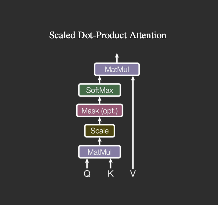
Figure 7: Scaled dot-product attention: queries and keys are multiplied, scaled by $\frac{1}{\sqrt{d_k}}$ normalized with softmax (optionally masked), and used to weight the values. Credit: Vaswani et al. [6].

Scaled dot-product attention is the core building block of the Transformer, and can be viewed as a mathematical refinement of Luong-style dot-product attention, vectorized for efficiency.

The computation is defined as:

Here, $Q$ represents queries, $K$ represents keys, $V$ represents values, and $d_k$ represents the dimension of the key vectors.

Using the dot product as a similarity measure is both conceptually natural and computationally efficient: the dot product captures how well each query aligns with each key, and it can be implemented as a single matrix multiplication across all tokens, making it highly GPU-friendly.

As explained by Vaswani et al. [6], the scaling factor, $1/\sqrt{d_k}$, is an important refinement. Without it, the magnitude of the dot products grows with the dimensionality of the keys, which can push the softmax into regions where gradients become very small, slowing learning. By scaling the dot products, the values remain in a stable range, improving gradient flow and training stability.

From a conceptual perspective, scaled dot-product attention generalizes Luong-style attention. In the RNN setting, Luong attention computes a dot product between a decoder hidden state and each encoder hidden state to determine relevance. Scaled dot-product attention extends this idea to handle sets of queries and keys simultaneously, allowing fully vectorized computation across sequences. In essence, it is global attention in matrix form, providing a stable, efficient, and parallelizable mechanism for computing relationships between tokens in both self-attention and encoder-decoder attention.

5.4Intuition & Example

Up to this point, attention has been described in terms of queries, keys, values, and matrix operations. But the mechanism itself is easier to understand if we step away from the notation and look at what it is doing at a token level.

At each position, the model is asking a simple question:

given the current token, which other tokens in the sequence are relevant right now?

The Query, Key, and Value formulation is just a way to parameterize this process:

• Query ($Q$): what the current token is trying to find
• Key ($K$): how other tokens expose what they contain
• Value ($V$): what actually gets pulled once a match is made

For a given token, attention computes a compatibility score between its query and all keys, normalizes these scores into a probability distribution, and uses them to form a weighted combination of the values. In effect, the token “looks at” all other tokens and selectively gathers relevant information.

5.4.1 A concrete example

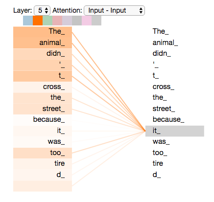
Figure 8: Self-attention allows the model to focus on “animal” when processing “it”. Credit: Alammar [4].

Consider the sentence:

“The animal didn’t cross the street because it was tired.”

When processing the token “it”, the model needs to determine what it refers to.

The query corresponding to “it” is compared with the keys of all tokens in the sentence (see Figure 8). Tokens like “animal” receive higher scores because their representations are more compatible with the query, while tokens like “street” or “cross” receive lower scores.

After applying softmax, this produces a distribution over all tokens. The context vector for “it” is then a weighted combination of all token representations, with most of the weight placed on “animal”. As a result, the representation of “it” now encodes information about “animal”, allowing the model to resolve the dependency.

There is no explicit rule for coreference here — the behavior emerges from how the model learns to assign these weights.

5.4.2 From sequences to structures

The deeper shift introduced by self-attention is structural. In RNNs, tokens interact through a chain. Each hidden state depends on the previous one, so information must flow step by step. This makes long-range dependencies difficult, as signals from earlier tokens must pass through many intermediate steps.

In encoder-decoder attention, this is partially relaxed: the decoder can directly access all encoder states. However, the encoder itself is still built sequentially, so the underlying representation still carries this limitation.

In self-attention, the sequence becomes a fully connected graph. Every token has a direct path to every other token within a layer. This reduces the path length between any two tokens to $O(1)$, enabling efficient modeling of long-range dependencies. Instead of relying on hidden state propagation, relationships are computed explicitly through pairwise interactions.

A useful way to think about this is:

instead of processing tokens sequentially, the model computes all pairwise relationships and then aggregates them.

This shift — from sequential computation to direct interaction — is what enables Transformers to model long-range dependencies efficiently while remaining fully parallelizable during training.

6Conclusion

The development of attention can be seen as a sequence of attempts to address a single issue: how to represent and access information from variable-length sequences.

Early approaches such as RBMT and SMT treated alignment and translation as separate components, relying on hand-crafted rules or probabilistic heuristics. Sequence-to-sequence models unified these steps into a single neural framework, but introduced a new bottleneck by compressing the entire input into a fixed-dimensional representation.

Attention relaxed this limitation by allowing the model to access different parts of the input dynamically during decoding. Instead of relying on a single context vector, the model computes a context at each step, turning alignment into a learned and differentiable operation. This removed the compression bottleneck. However, the underlying computation remains sequential due to the use of RNNs.

The next step was to remove this remaining constraint. If attention already allows direct access to all relevant information, then recurrence is no longer necessary. Self-attention extends this idea by allowing all tokens in a sequence to interact directly, eliminating sequential dependencies in the architecture. Scaled dot-product attention provides an efficient and stable way to compute these interactions, enabling fully parallel computation.

From this perspective, the Transformer is not a sudden innovation, but a natural consequence of this progression. Each step — encoder-decoder models, attention, and self-attention — removes a specific limitation of the previous approach, gradually shifting from implicit, sequential representations to explicit, parallel interactions.

Mechanisms such as multi-head attention build on this foundation by allowing the model to capture multiple types of relationships in parallel, but they do not change the core idea.

In summary, attention reframes sequence modeling from compressing information to selectively retrieving it, and self-attention completes this transition by making all interactions explicit and parallel. This shift in perspective is what enables the effectiveness of modern Transformer-based models.

Notes

1. Note that Ilya et al. passed the input sequence in reverse, so inputs “ABC” were feed “C”, “B”, “A” order. Initially they thought reversing the input sentences would result in more confident predictions in early parts of target sentences and less confident predictions in later parts. But surprisingly it performed much better on long sentences. They did not have an explanation for this phenomenon, but they believe that it is create many short term dependencies to the dataset. The LSTM’s test perplexity dropped from 5.8 to 4.7 and the test BLEU scores of its decoded translations increased from 25.9 to 30.6.

References

1. Ilya Sutskever, Oriol Vinyals, and Quoc V. Le, Sequence to Sequence Learning with Neural Networks, arXiv:1409.3215, 2014. https://arxiv.org/abs/1409.3215 ↑¹ ↑²

2. Dzmitry Bahdanau, Kyunghyun Cho, and Yoshua Bengio, Neural Machine Translation by Jointly Learning to Align and Translate, arXiv:1409.0473, 2016. https://arxiv.org/abs/1409.0473 ↑¹ ↑² ↑³ ↑⁴ ↑⁵ ↑⁶

3. Kyunghyun Cho, Bart van Merrienboer, Dzmitry Bahdanau, and Yoshua Bengio, On the Properties of Neural Machine Translation: Encoder–Decoder Approaches, arXiv:1409.1259, 2014. https://arxiv.org/abs/1409.1259 ↑

4. Jay Alammar, The Illustrated Transformer, 2018. https://jalammar.github.io/illustrated-transformer/

5. Minh-Thang Luong, Hieu Pham, and Christopher D. Manning, Effective Approaches to Attention-based Neural Machine Translation, arXiv:1508.04025, 2015. https://arxiv.org/abs/1508.04025 ↑¹ ↑² ↑³ ↑⁴ ↑⁵

6. Ashish Vaswani, Noam Shazeer, Niki Parmar, Jakob Uszkoreit, Llion Jones, Aidan N. Gomez, Lukasz Kaiser, and Illia Polosukhin, Attention Is All You Need, arXiv:1706.03762, 2023. https://arxiv.org/abs/1706.03762 ↑

7. Kelvin Xu, Jimmy Ba, Ryan Kiros, Kyunghyun Cho, Aaron Courville, Ruslan Salakhutdinov, Richard Zemel, and Yoshua Bengio, Show, Attend and Tell: Neural Image Caption Generation with Visual Attention, arXiv:1502.03044, 2016. https://arxiv.org/abs/1502.03044 ↑

Citation

If you found this post useful, please cite it as:

@online{meena2026attention,
  author  = {Abhijeetsingh Meena},
  title   = {Understanding Attention by Tracing Its Origins},
  year    = {2026},
  url     = {https://abhijeetmeena.com/blog/understanding-attention-by-tracing-its-origins},
  urldate = {2026-03-29}
}